The Landau Distribution and Energy Loss For Ionizing Particles

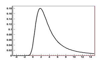
A charged particle crossing a silicon sensor does not deposit the average amount of energy. It deposits whatever a handful of random collisions happen to give it — usually less than the average, occasionally very much more. Design a readout chip around the mean and you will mis-set the threshold on almost every event.

That is the practical content of the Landau distribution. Bethe-Bloch tells you the mean energy loss; Landau, in 1944, told you how wildly individual events scatter around it — and why the mean is the wrong number to build hardware on.

The Bethe-Bloch formula is well recognised for describing the average energy loss of charged particles passing through matter, whereas Landau theoretically described the fluctuations of energy loss by ionisation of a charged particle in a thin layer of matter in 1944 [1]. This description concludes with Landau Distribution, a universal asymmetric probability density function.

Why the peak sits below the mean

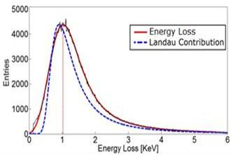
In reality, if a particle does not stop in the sensor, the response ranges around the distribution’s peak, with a high possibility of strong signals. Because of this tail, the average value exceeds the distribution’s most probable value. The variation around the maximum of this distribution increases as the sensor gets thinner. When constructing the readout circuit for these devices, the dynamic range must be considered.

Knock-on electrons: where the tail comes from

The Landau fluctuation is principally induced by the uncommon but measurable occurrence of knock-on electrons, which gain enough energy from the contact to become ionising particles themselves. The direction of the knock-on electron is often perpendicular to the direction of the incoming particle, resulting in uneven charge clouds and reduced spatial resolution.

The convolution property

The convolution of two Landau distributions results in another Landau distribution. This property can be illustrated by the energy loss of a particle traversing a layer of thickness D or two subsequent layers of thickness D/2, respectively. The overall energy loss must be the same in both cases, implying the convolution property mentioned above.

Although the Landau distribution has a finite area, it is impossible to calculate mean values due to the infinite tail. One proposed remedy is to cut the Landau tail, which would result in the loss of the convolution characteristic.

Protons, pions and other types of charged particles, which are in most cases close to MIPs, all produce approximately Landau-distributed spectra when traversing the matter. There are several approximations; the simplest is to apply the Gaussian function if the goal is to fit only the most probable value (peak).

The first and second momenta Φ (1,x) and Φ (2, x) of the density function truncated on the right-hand tail can be defined through the general formula

When Landau applies — and the assumptions behind it

It is possible to use the Landau function for all situations where k < 0.01 (where k is the ratio of the mean energy loss and the Maximum Transferable Energy) with the assumptions that:

• The maximum energy transfer is infinite
• The electron binding energy in a collision is negligible, in other words, the electrons involved in collisions are treated as free and the distant collision is ignored
• The particle velocity remains approximately the same
• Taking only the first term of Bethe-Block formula, the mean energy loss is approximated to:

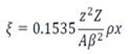
The Landau distribution is then given by:

r is an arbitrary real constant and the variable l is:

where C_E is the Euler constant. The function φ(λ) is a universal function that must be evaluated numerically. A tabulation for various λ can be found in some articles. In addition, computer program has been developed and can be found here (Matlab code). 

The most probable energy loss

The φ(λ) has a maximum for a λ of 0.229 and a full width at half maximum: W_L=4.02ξ. The energy loss corresponding to the maximum of the function f_L(x,Δ) is called the most probable energy loss ( Δ_p).

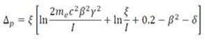
Earlier values for the constant 0.2000 were 0.37 [1] and 0.198 [3]. The equation includes the density effect, which had not been used by Landau.

For γ >> 100, we get

Δ_p= ξ ( 12.325 + ln(ξ/I) )

If we enter the I value, we obtain

Δ_p(keV) = t (0.1791 + 0.01782 lnt ) with t in um.

Where Landau breaks down: very thin absorbers

For small thicknesses, the Landau fails to fit the experimental energy loss distribution [2]. In fact, for small thicknesses, the Landau shows a lower position of the peak with respect to the energy loss distribution measured (Fig. 2(a)).

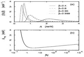It can be understood qualitatively: for very thin absorbers, K-shell electrons do not contribute to the energy loss. Thus, the effective thickness of the absorber can be considered to be t_e=12/14 t. For t = 10 um, t_e=8.57 um.

The full width at half maximum of the Landau function, w, depends on the absorber thickness and is independent of particle type and speed.

References

1. L. Landau, On the Energy Loss of Fast Particles by Ionization, J. Phys. USSR 8 (1944) 201.
2. Blunck and S. Leisegang, Zum Energieverlust schneller Elektronen in d nnen Schichten, Z. Physik 128 (1950) 500.
3. Maccabee and Papworth (1969), quoted by Sternheimer and Peierls (1971); see, also, Ahlen (1980)

If you want the experimental side of this — what the measured distributions actually look like in thin silicon, and where the Landau prediction parts company with them — that is covered in the straggling function. For what happens to the liberated charge once it exists, see charge carrier generation in semiconductors.