The statistical nature of the ionising process during the passage of a fast charge particle through matter results in large fluctuations in the energy loss (Δ) in absorbers, whose thickness is thin compared to the particle range.
The number of electron-hole pairs (J) is related to Δ by the expression J=Δ/P, where P is a proportional factor, which for silicon equals 3.68 eV. Both Δ and J are stochastic quantities. The probability functions f(Δ) and φ(J) are usually called energy loss distribution or straggling functions.
They can be described schematically by the position of the maximum of distribution function (Δp) and the full width at half maximum (w), with Δp being located at lower value compared to the mean energy loss obtained from Bethe-Bloch ‹Δ› (Fig.1).
(click here to download the C++ Bethe-Bloch calculator).
The mean energy loss: Bethe-Bloch
The collisions are casual, of course, but their number per macroscopic path length is generally large and this is the reason why average quantities are generally used. One of the most important quantity is the mean energy loss per units length, often called stopping power. Many theories have been developed during the first half of the twentieth century in order to characterize this quantity. The correct quantum‑mechanical calculation was first described, around 1932, by Hans Bethe, Bloch and other authors who gave the formula:

with:
| 2π Na re^2 mec^2= 0.1535 MeVcm2/g | β: v/c of incident particle |
| re: electron radius (2.817 x 10⁻¹³ cm) | ρ: density of absorbing material |
| Me: electron mass | γ:  |
| Na: Avogadro’s number | δ: density correction |
| Z: atomic number of absorbing material | C: shell correction |
| A: atomic weight of absorbing material | I: mean excitation potential |
| z: charge of incident particle | Wmax: maximum energy transferable in a single collision |
Wmax can be calculated using the equation:
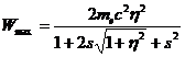
where: s=me/M and η=βγ.
The mean excitation energy I depends by the orbital frequency of the absorbing material and there is not a precise formula to calculate that value. However values of I for several material have been deduced from measurements and are tabulated by the ICRU. The last two terms in the parentheses of the formula are the density and the shell corrections and they have been inserted in the original formulation of Bethe‑Bloch in order to enhance the prediction of the formula at certain range compared to the experimental results. The density correction takes into account the effect of the electric field produced by incoming particles and is more evident at high velocity. Instead, the shell correction is noticeable when the velocity of incident particle is comparable to the orbital velocity of the bound electrons of the target material.
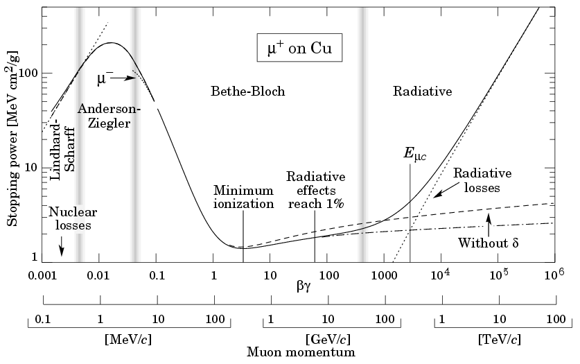
At this low energy some other complicated effects come into play and the Bethe-Bloch formula breaks down. When the velocity is comparable with the speed of orbital electrons of the target material the energy loss reach a maximum depending on the sign of the charge (Barkas effect) and for lower energy drops sharply. At higher energy (that means higher velocity) dE/dx is dominated by the 1/β2 factor and decreases until β ≅ 0.96c where a minimum is reached. Particle with this energy is usually indicated with the name of minimum ionizing particle (MIP).
Increasing the energy the losses do not increase so much due to the density effect (Fermi plateau) until the radiative components, such as the Cherenkov radiation and Bremsstrahlung, start to be relevant. The Cherenkov radiation arises when a charged particle in a medium moves faster than the speed of light in that same medium (βc>c/n, with n: index of refraction): in such case an electromagnetic shock wave is created, just as an aircraft that moves faster than sound.
Especially for light particles, such as electrons or positrons at very high energy, the Bremsstrahlung emission represents the main energy loss mechanism. The deflection and the deceleration of the particle due to the interaction with the nuclei of the target cause the emission of photons; this effect is much greater as lighter is the particle (in fact the emission probability by Bremsstrahlung varies as the inverse square of the particle mass) and higher is the atomic number of target material. While ionization loss rates rise logarithmically with energy , Bremsstrahlung losses rise linearly and dominate at high energy (just only above few tens of MeV in most material for electrons). Fig. 1 below shows the mean energy loss (the stopping power) for positive muons in copper, from a few hundred keV to tens of TeV.
Correction to Bethe-Bloch for electrons and positrons
Electrons or positrons needs particular consideration. First, their small mass implies the possibility of a large deflection due to a single collision too; moreover the collisions are between identical particles, so that the calculation must take into account their indistinguishability. As result the maximum transferable energy in a single collision becomes:

with Te: kinetic energy of the incident particle, and the Bethe-Bloch formula can be rearranged as:
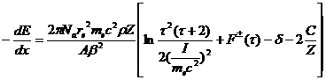
with:

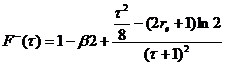

where suffix “+” means positrons and “–” means electrons.
From the mean to the distribution: Landau and Vavilov
Landau and Vavilov performed theoretical calculations on this distribution. Each of these solutions, however, has a different region of applicability and the distinguishing parameter in all these theories is the ratio k = ‹Δ› / Emax where Emax is the maximum transferable energy in a single collision.
Landau solved this problem for all situations where k ≤ 0.01, deriving the expected energy loss distribution by solving an integral transport equation:

Here f(x,Δ) represents the distribution probability that the incident particle will lose an amount Δ of energy on traversing a layer of thickness x. W(E)dE denotes the probability per unit path length of a collision transferring energy E to an electron in the material.
The function W(E)dE is not generally known, but Landau was able to derive an approximate solution by using the free electron (Rutherford) cross section:

with

keV μm-1 in silicon.
In the previous equation, z is the charge of the incident particle, Z and A are the atomic number and weight of the material, and ρ is the density. The Landau distribution is therefore given by [1]

with φ(λ) a universal function of the variable λ only
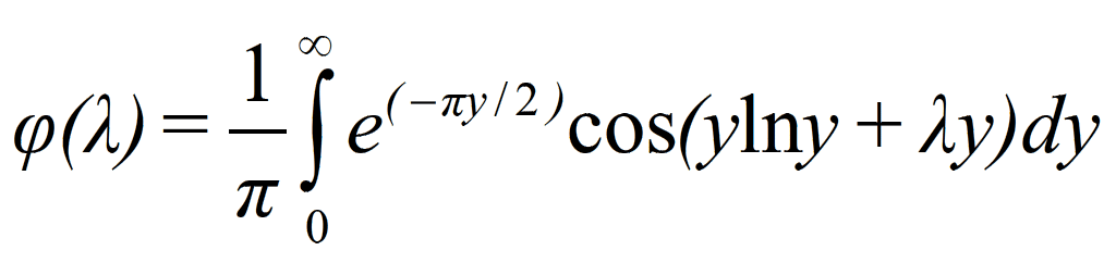
and
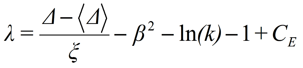
where CE is the Euler constant equal to 0.5772. The Landau distribution, fL(Δ), is asymmetric with a tail extending to Emax with a maximum for λ=-0.229 and w=4.018ξ. This tail is mainly due to fast-emitted δ-rays. The energy loss corresponding to the maximum of the function fL(Δ) is the most probable energy loss [2]

where I is the mean excitation potential and δ is the density correction. (click here to download the Matlab Landau Fit)

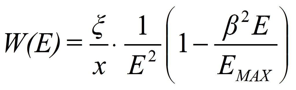
Subsequently, Vavilov [3] derived an improved solution that takes into account the spin of the incident particle and introduces the physical limits coming from Emax. For the collision cross-section, Vavilov used the form

Interaction of Particles with Matter: From Theory to Measurements
Understand the Mysteries of Radiation: Master the Interaction with Matter in a Few Simple Steps
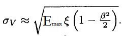
Vavilov also demonstrated that his solution tends to the Landau function for k ≤ 0.01, region where ‹Δ› is approximated to ξ. For instance, for 300 um silicon detectors, the convergence is already achieved by protons with momenta larger than 550 MeV/c. For k > 10, the number of collision is very large and, for the Central Limit Theorem, the Vavilov function coincides with Gaussian distribution, where the standard deviation is

Get the next one by email
Physics, engineering and the people behind them. No spam, unsubscribe any time.
Binding corrections: why the measured width is broader
Landau-Vavilov solutions have been derived under the assumption that scatterings occur on quasi-free electrons. Therefore, they neglect the electron-binding energies. This assumption is a valid approximation only for close collisions.
Further corrections to the theory, taking into account the fact that the electrons in the material are not free, have been attempted by Blunck and Leisegang [4], Shulek [5] and Bichsel [6].
In the case of solid media, these calculations are aimed at the experimental observation that, while the most probable energy loss agrees rather well with the prediction of the theory, the width of the distribution is broader than expected and cannot be accounted for by electronic noise or imperfect resolution. The effect is particularly noticeable for very thin absorbers [7], of the order of a few hundred μm or less. The modified energy loss distribution can be improved by using a modified cross section to take into account the electron binding energy and the atomic shell structure. The modified energy straggling function can be expressed as:
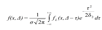
In other words, the experimentally observed energy spectrum can be calculated by convoluting the Landau distribution with a normal distribution of variance δ2. The result of the convolution is a broader distribution with a peak value that is usually increased by a small amount compared to the Landau theory. From the experimental observations, the δ2 value has been estimated:
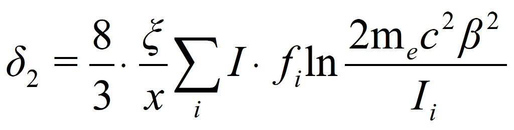
where fi is the fraction of electrons in that shell. In silicon, this approaches a value of

The resulting improved energy loss distribution has an overall value of w, which is roughly given by:
√[(4.018 ξ )^2 + ( 5.56 δ2 )]
As the material thickness decreases, δ2 becomes more and more the dominant term, which determines the overall w of the straggling function. Conversely, it is not expected to provide an additional broadening of the distribution at large thicknesses.
As an example, in a 300 μm thick silicon detector, we get ξ is ~ 5.34 keV, √(δ2) is ~ 5.76 keV, and an overall w is 25.4 keV (i.e., 18% larger than Landau width) for a relativistic β~ 1 and z = 1 particle in agreement with the experimental data.

Reference tool
Energy-loss calculator: mean, most probable value and straggling
Your particle, your absorber. Mean rate from the Bethe formula with the density-effect correction, the most probable loss from the Landau theory as given in the PDG review, and the straggling curve for your case.
The calculator needs JavaScript. The reference values below are computed by the same code.
Method, constants and limits
Method. Mean rate: Bethe formula, ⟨−dE/dx⟩ = K z² (Z/A) β⁻² [ ½ ln(2mec²β²γ²Tmax/I²) − β² − δ/2 ], without shell or Barkas terms (they exceed a few percent only below βγ ≈ 0.1). Most probable loss: Δp = ξ [ ln(2mec²β²γ²/I) + ln(ξ/I) + 0.200 − β² − δ ], ξ = (K/2) z² (Z/A) x/β². Regime from κ = ξ/Tmax: Landau below 0.01, Vavilov to 10, Gaussian above. The Landau density is evaluated by direct quadrature of its defining integral, not an approximation. Both formulas and their notation follow the Particle Data Group review Passage of particles through matter.
Electron-hole pairs (silicon only). Pairs per micrometre = energy deposited per micrometre ÷ w, w = 3.62 eV (silicon, room temperature; PDG review / silicon-detector literature, e.g. Knoll, Radiation Detection and Measurement). Two figures are reported, not one, because they answer different questions: the mean rate uses ⟨dE/dx⟩ and does not depend on thickness (≈108/µm for a minimum-ionising particle in silicon); the most probable rate uses Δp at the thickness entered above and does depend on it, because Δp is not linear in thickness — it is what a thin detector actually reads out on a single pass, the same Landau/straggling quantity this tool otherwise reports in keV. Quoting only the mean figure for a thin-detector signal is a common error this tool deliberately avoids.
Constants. I, density, Z/A and δ(βγ) per material from NIST ESTAR (SRD 124); K = 4πNAre²mec² and mec² from CODATA; particle masses from the PDG; w = 3.62 eV for silicon as above — not an ESTAR/XCOM quantity, typed directly in the engine with its source. The Bethe engine reproduces NIST PSTAR proton stopping powers to within 1% from 50 MeV to 10 GeV in every material offered; the deviations are on record in the repository tests.
Limits. Heavy charged particles only (no electrons). βγ from 0.1 to about 2×10⁴. Thin absorbers: when the mean loss exceeds 10% of the kinetic energy the constant-velocity assumption fails and the result says so. The e-h pair figures are silicon-only: no sourced w is offered for any other material.
Reference values: a minimum-ionising muon in silicon
Muon at βγ = 3.5 (369.8 MeV/c), where the mean rate in silicon is at its minimum. Computed by the calculator above. The last two columns are the e-h pair yield per micrometre (w = 3.62 eV): the most-probable column changes with thickness because Δp is not linear in x; the mean column does not.
| Thickness (µm) | Most probable loss Δp (keV) | Mean loss (keV) | FWHM (keV) | Δp / mean | κ | e-h pairs/µm (most probable) | e-h pairs/µm (mean) |
|---|---|---|---|---|---|---|---|
| 50 | 11.31 | 19.33 | 3.876 | 0.585 | 8.0e-5 | 62.48 | 106.8 |
| 100 | 23.96 | 38.65 | 7.751 | 0.62 | 1.6e-4 | 66.17 | 106.8 |
| 150 | 37.11 | 57.98 | 11.63 | 0.64 | 2.4e-4 | 68.34 | 106.8 |
| 200 | 50.58 | 77.3 | 15.5 | 0.654 | 3.2e-4 | 69.87 | 106.8 |
| 300 | 78.22 | 116 | 23.25 | 0.675 | 4.8e-4 | 72.03 | 106.8 |
| 500 | 135.3 | 193.3 | 38.76 | 0.7 | 8.0e-4 | 74.75 | 106.8 |
| 1000 | 284 | 386.5 | 77.51 | 0.735 | 1.6e-3 | 78.44 | 106.8 |
Method: PDG review Passage of particles through matter (Bethe formula, Landau most probable value). Constants: NIST ESTAR silicon (I = 173 eV, ρ = 2.33 g/cm³), CODATA, PDG masses. Pair-creation energy w = 3.62 eV (silicon, room temperature; PDG review / silicon-detector literature) is not an ESTAR/XCOM quantity and is typed directly in the engine.
Minimum ionisation by material
The minimum of the mean rate ⟨−dE/dx⟩ for a singly charged heavy particle, and the βγ at which it occurs.
| Material | ρ (g/cm³) | I (eV) | Z/A | βγ at minimum | ⟨−dE/dx⟩min (MeV cm²/g) | (keV/µm) |
|---|---|---|---|---|---|---|
| Silicon | 2.33 | 173 | 0.4985 | 3.42 | 1.659 | 0.3865 |
| Germanium | 5.323 | 350 | 0.4408 | 3.26 | 1.372 | 0.7301 |
| Carbon (amorphous) | 2 | 81 | 0.4995 | 3.92 | 1.743 | 0.3486 |
| Aluminium | 2.699 | 166 | 0.4818 | 3.42 | 1.611 | 0.4347 |
| Iron | 7.874 | 286 | 0.4656 | 3.44 | 1.45 | 1.142 |
| Copper | 8.96 | 322 | 0.4564 | 3.42 | 1.402 | 1.257 |
| Tungsten | 19.3 | 727 | 0.4025 | 3.16 | 1.144 | 2.207 |
| Lead | 11.35 | 823 | 0.3958 | 3.02 | 1.121 | 1.273 |
| Argon (gas) | 0.001662 | 188 | 0.4506 | 3.16 | 1.519 | 2.524e-4 |
| Water | 1 | 75 | 0.5551 | 4 | 1.998 | 0.1998 |
| Air (dry, sea level) | 0.001205 | 85.7 | 0.4992 | 3.3 | 1.815 | 2.186e-4 |
| Plastic scintillator | 1.032 | 64.7 | 0.5414 | 4.04 | 1.956 | 0.2018 |
| Kapton | 1.42 | 79.6 | 0.5126 | 3.96 | 1.82 | 0.2584 |
| Silicon dioxide | 2.32 | 139.2 | 0.4993 | 3.64 | 1.697 | 0.3937 |
| Concrete (Portland) | 2.3 | 135.2 | 0.5027 | 3.66 | 1.711 | 0.3936 |
| Bone (compact, ICRU) | 1.85 | 91.9 | 0.5301 | 3.92 | 1.849 | 0.3421 |
| Soft tissue (ICRP) | 1 | 72.3 | 0.5512 | 4.02 | 1.985 | 0.1985 |
Bethe formula with the NIST ESTAR density-effect correction; no shell or Barkas terms. Material constants: NIST ESTAR (SRD 124). Checked against NIST PSTAR to within 1% (50 MeV – 10 GeV protons).
Prefer a bare calculator, or want the electron-hole pair yield per micrometre for your own case? Open the energy-loss tool on its own page →
References
- L. Landau , On the Energy Loss of Fast Particles by Ionization, J. Phys. USSR 8 (1944) 201.
- Particle Data Group PDG, Passage of particles through matter, Nuclear and Particle Physics, vol. 33, no. 27, pp. 258-270, July 2006.
- P.V.Vavilov, Ionization losses of high energy heavy particles, Soviet Physics JETP, 5:749, 1957.
- S. Meroli et al., Energy loss measurement for charged particles in very thin silicon layers , JINST, 6 P06013 doi: 10.1088/1748-0221/6/06/P06013
- Blunck and S. Leisegang, Zum Energieverlust schneller Elektronen in d�nnen Schichten, Z. Physik 128 (1950) 500.
- P. Shulek at al., Fluctuations of Ionization Loss, Sov. J. Nucl. Phys 4 (1967) 400.
- H. Bichsel, Straggling of Heavy Charged Particles: Comparison of Born Hydrogenic-Wave-Function Approximation with Free-Electron Approximation, Phys. Rev. B1 (1970) 2854
- H. Esbensen at al., Random and channeled energy loss in thin germanium and silicon crystals for positive and negative 2-15-GeV/c pions, kaons, and protons, Phys. Rev. B18 (1978) 103939
- William R. Leo, Techniques for Nuclear and Particle Physics Experiments. Berlin and Heidelberg: Springer, 1987.
- Claude Leroy, Pier Giorgio Rancoita, Principles of Radiation Interaction in Matter and Detection. Singapore: World Scientific Publishing, 2004.
- International Commission on Radiation Units and Measurements. [Online]. http://www.icru.org/
- S. M. Sze, Kwok Kwok Ng, Physics of Semiconductor Devices. John Wiley & Sons, 2007.
One story like this, most days
Written by a CERN physicist. No spam, unsubscribe any time.